Probability Distributions
In several areas of the software, such as load cycle inputs, users can apply a probability distribution to model variability and uncertainty. When actual data isn't available, you can provide estimates, or use historical data to represent real-world conditions. This flexibility ensures a more realistic simulation, improving accuracy.
Creating a Distribution
To create a basic probability distribution, you need at least three key parameters: the mean (average), minimum, and maximum values. By specifying these three parameters, you can define a range that encompasses all possible values, while the mean helps describe the likely center of this range. Depending on the distribution type, additional details like the standard deviation, skewness, or probability weights may further refine how data is spread between the minimum and maximum.
Mean
The mean in a probability distribution serves as the central point around which values are distributed. It represents the average of all possible outcomes, providing a useful summary of the distribution's overall tendency. In simulations, the mean helps to establish a baseline for expected values, allowing for a clearer understanding of variability and uncertainty in the data. By defining the mean, users can better assess how other parameters, such as minimum and maximum values, interact with the central tendency of the distribution.
To calculate the mean, add all the possible values together and then divide the total by the number of values.
Example: If you have the values 3, 5, and 7, the mean calculation would be:
Mean = (3 + 5 + 7) / 3 = 5
Min/Max
The minimum and maximum values need to be specified to define the range of possible outcomes for the probability distribution. This ensures that the simulation only considers values within realistic limits, helping to avoid extreme or improbable results. By setting these boundaries, you create a more accurate representation of variability within the specified range. There are two different methods, percentage and absolute, which are detailed below.
Percentage
In this method, the min and max values are calculated as percentages of the specified mean. The software determines these values based on the defined min and max percentages, indicating how far below or above the mean the values can range. This approach allows for a flexible distribution that accurately reflects the potential variability while remaining proportional to the central value.
The following inputs are required.
| Input | Description |
|---|---|
| Mean | This mean represents the central value of the distribution |
| Min Percentage | The minimum value of the distribution, expressed as a percentage of the mean. |
| Max Percentage | The maximum value of the distribution, expressed as a percentage of the mean. |
Example: If the Mean is set to 8, the Min Percentage is set to 100%, and the Max Percentage is set to 300%:
-
Minimum Value = Mean * (Min Percentage / 100) = 8 * (100 / 100) = 8
-
Maximum Value = Mean * (Max Percentage / 100) = 8 * (300 / 100) = 24
Absolute
In this method, the min and max values are directly specified based on actual numerical inputs. In this case, the software utilises the provided minimum and maximum values to establish the range for the probability distribution. This approach allows for precise control over the distribution, reflecting specific operational constraints or historical data while ensuring that the variability is bounded within the defined limits.
| Input | Description |
|---|---|
| Min | The minimum value of the distribution. |
| Max | The maximum value of the distribution. |
Distribution Types
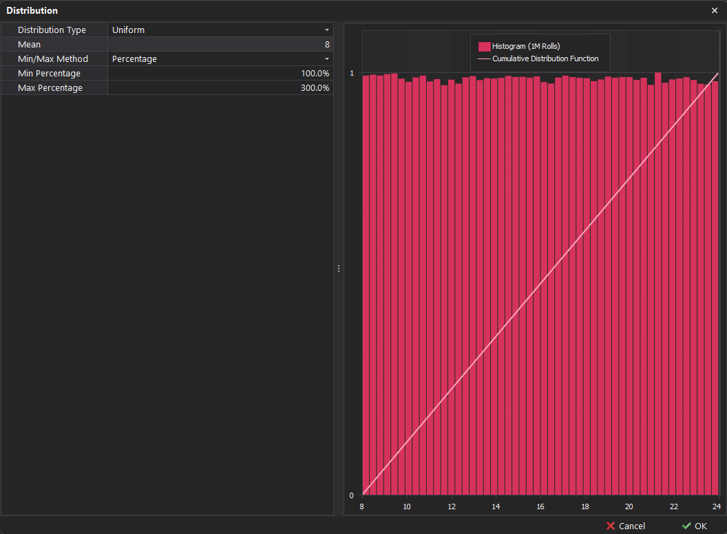
Uniform
A uniform distribution is a probability distribution in which all outcomes are equally likely within a specified range. This type of distribution is useful for modeling variables with consistent probabilities.
🎲 Example - Consider the possible outcomes of rolling a 6-sided die : 1, 2, 3, 4, 5, or 6. In this scenario, each of the six numbers has an equal chance of being rolled.
The histogram below, which uses the 'Percentage' method, visually shows this type of distribution.
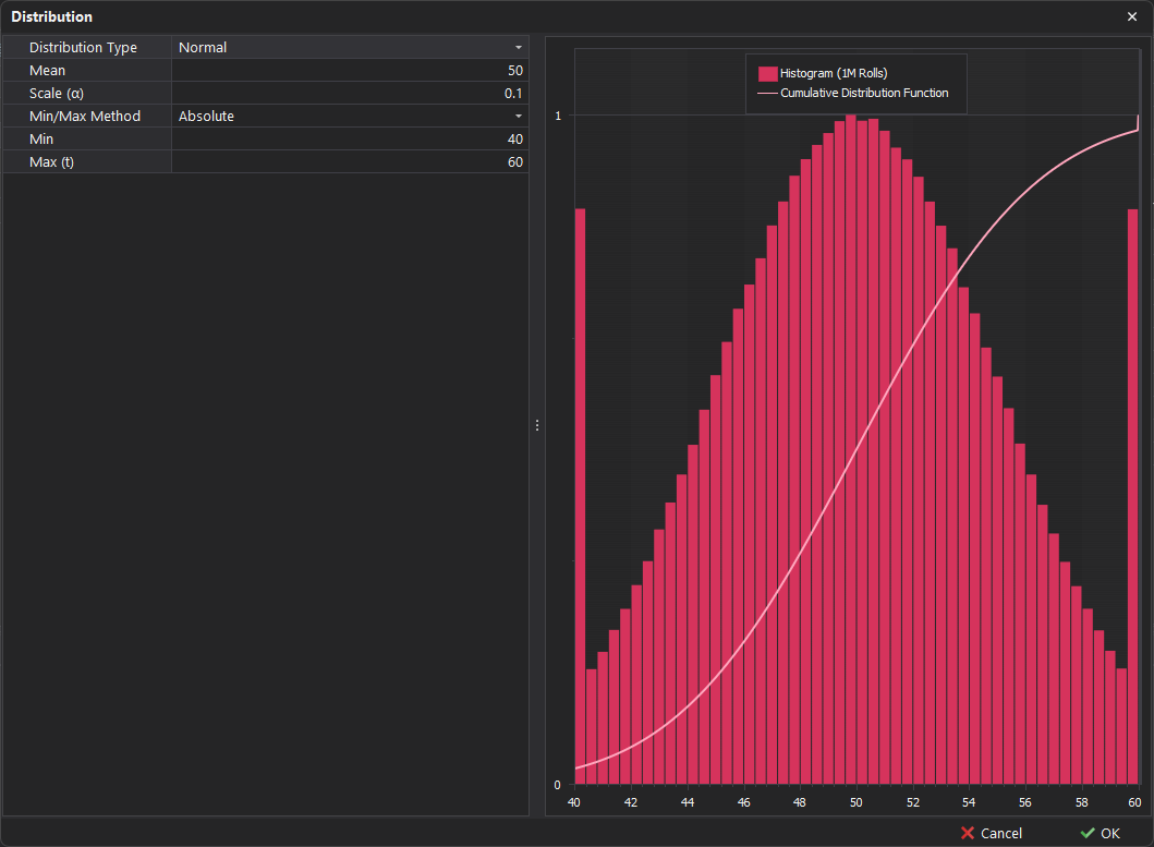
Normal
A normal distribution is a probability distribution that is symmetric around the mean, with most data points clustering near the center and tapering off toward the extremes.
🪣 Example - The average bucket payload is 50 tonnes, with most instances falling within a few tonnes above or below this average.
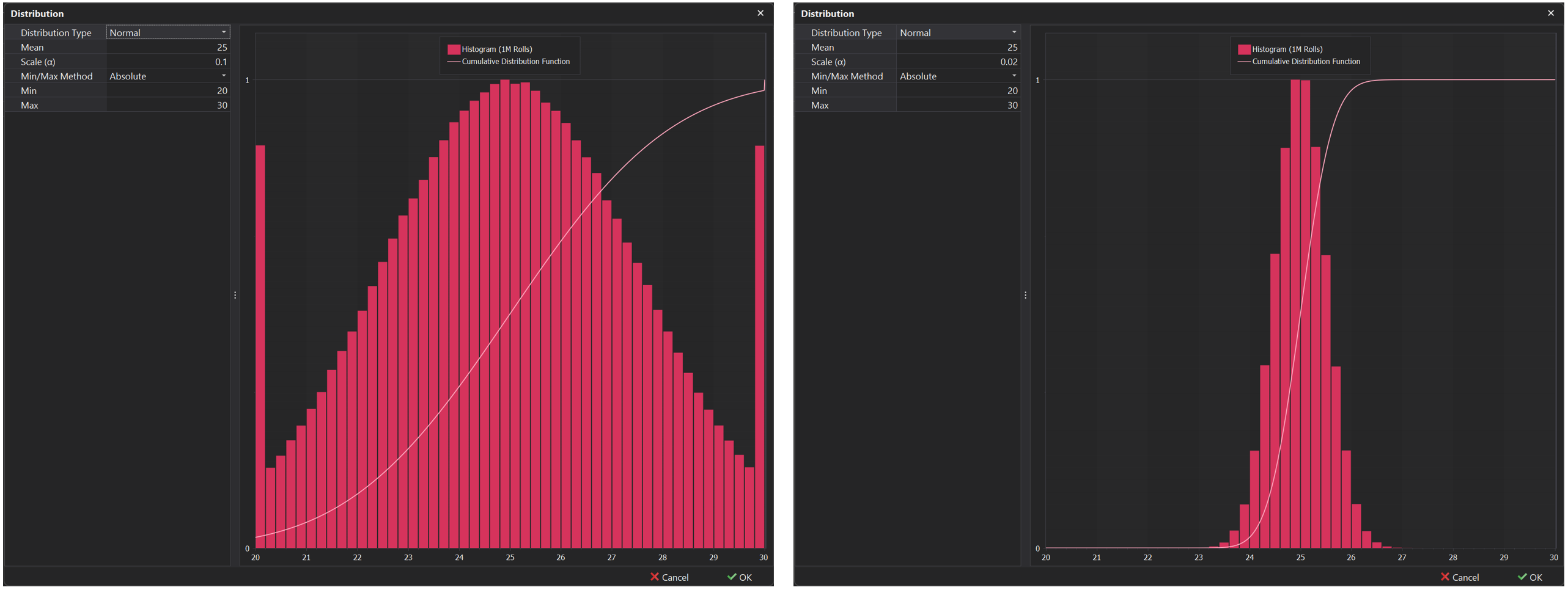
Scale (α)
In this type of distribution, an additional Scale input appears, denoted by the character α, which can be used to control the standard deviation or variance. This defines how spread out or clustered the data points are around the mean. By adjusting the scale, you can increase or decrease the variability of the distribution, making it a useful tool for fine-tuning the level of uncertainty or dispersion.
Smaller Scale: A smaller scale value indicates lower variability, with values tightly clustered around the mean.
Larger Scale: A larger scale indicates higher variability, with values more spread out from the mean.
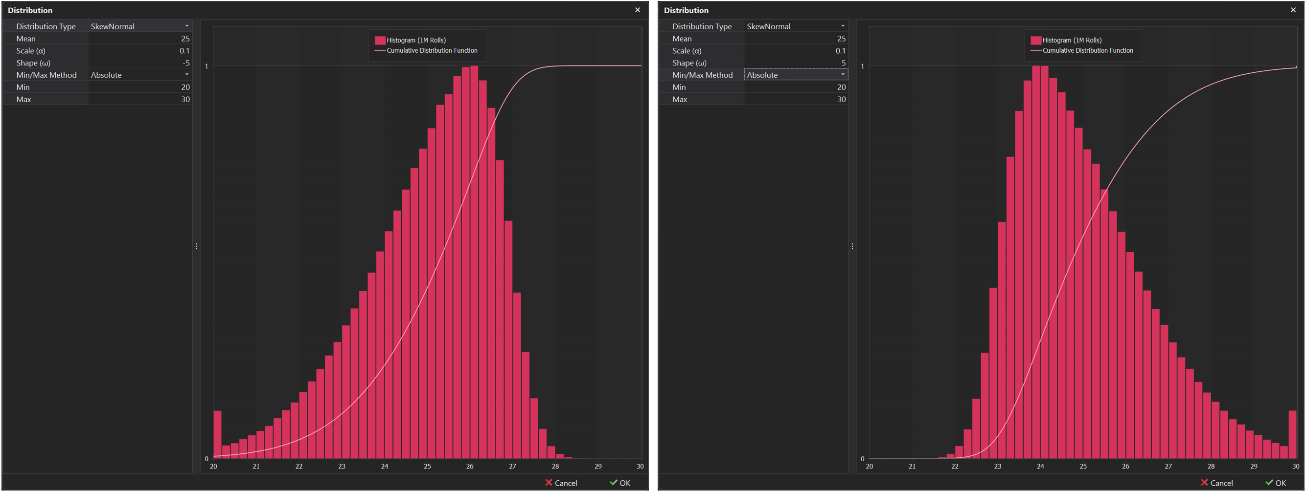
Skew Normal
Similar to the normal distribution, the skew-normal distribution introduces asymmetry (skewness) in the data, making it particularly valuable for modeling scenarios where the data deviates from symmetry. This distribution effectively captures variations in real-world datasets, allowing for a more accurate representation of situations where the outcomes are not evenly distributed around the mean.
⏱️ Example - If swing times are generally longer but occasionally experience shorter swings, a skew-normal distribution can effectively model this variability by capturing the asymmetry in the data.
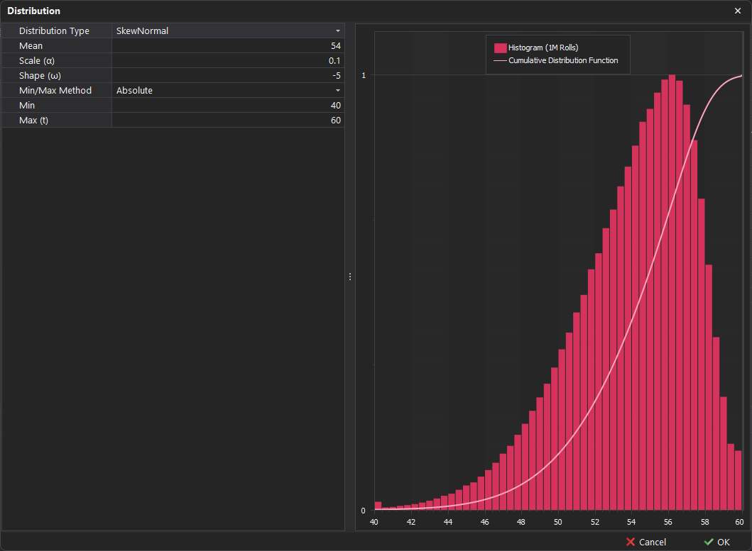
Shape (ω)
In addition to the scale input covered above in the Normal Distribution, an additional Shape input appears, denoted by the character (ω). This input controls the amount of skewness in the distribution.
Positive values - Will result in a Positive Skew where the distribution tail extends more to the right.
Negative Values - Will result in a Negative Skew where the distribution tail extends more to the left.